The problem
Military communications, radar and electronic-warfare systems depend on radio links that an opponent may try to jam deliberately. Suppressing that interference in real time is an operational requirement, not a nice-to-have, and adaptive filters are the standard tool for the job.
The report explains the structure of an adaptive filter and then examines two application environments where the same theory appears in different forms: adaptive phased-array beamforming in the spatial domain, and an LMS anti-jam filter in the time domain.
How an adaptive filter works
The general structure is a transversal FIR filter with adjustable tap weights, an error generator that compares the output with a desired reference, and a weight-update algorithm that minimises the mean-square error. The least-mean-squares algorithm updates the weights in proportion to the error and the input, with a step size that trades convergence speed against stability.
The step size must satisfy 0 < mu < 1/lambda_max, where lambda_max is the largest eigenvalue of the input autocorrelation matrix. Recursive least squares converges faster by minimising a weighted least-squares cost over all past samples, at the price of more computation.
Beamforming
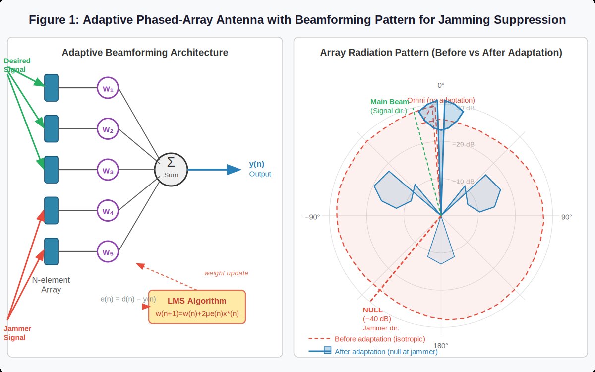
In a phased array, each element output is weighted and summed. The adaptive weights steer a high-gain main lobe toward the wanted signal and place nulls in the directions of interferers; an N-element array has N-1 adaptive degrees of freedom.
The data product is the beam pattern: array gain in dBi against angle. In the reported case the adapted pattern reaches roughly +15 to +20 dBi toward the wanted signal and a null of -40 dB or more toward the jammer, with 30–50 dB of suppression in operational systems. The convergence curve of MSE against iteration count is what engineers use to set the step size.
Anti-jam receiver
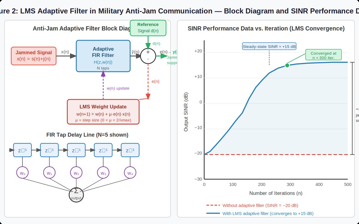
The time-domain case receives x(n) = s(n) + j(n), the wanted signal plus jamming. A locally generated reference, from a pilot sequence or a prediction of the wanted signal, drives the LMS filter to model and cancel the jammer.
Here the main data product is output SINR against iteration number. In the example the SINR rises quickly and reaches a steady state of about +15 dB after roughly 300 iterations, which corresponds to about 35 dB of jammer suppression. The residual jamming power spectral density shows the notch the filter has formed.
What the study shows
The two cases look different on a block diagram but share the same mechanism: use a reference to separate what you want from what you do not, and adapt until the error is small. The engineering difficulty is in the reference, the step size and the array or filter order that the hardware can afford.
Figures